Vehicle Choice Mixed Logit#
import pandas as pd

import larch as lx
from larch import PX
In this example, we will demonstrate the estimatation of parameters for mixed logit models. The examples are based on a problem set originally published by Ken Train.
To ensure good preformance and ease of use, estimating parameters for a mixed logit model in Larch requires the jax library as the compute engine. Importing it here allows us to confirm that it is available.
import jax # noqa: F401
The data represent consumers’ choices among vehicles in stated preference experiments. The data are from a study that he did for Toyota and GM to assist them in their analysis of the potential marketability of electric and hybrid vehicles, back before hybrids were introduced.
In each choice experiment, the respondent was presented with three vehicles, with the price and other attributes of each vehicle described. The respondent was asked to state which of the three vehicles he/she would buy if the these vehicles were the only ones available in the market. There are 100 respondents in our dataset (which, to reduce estimation time, is a subset of the full dataset which contains 500 respondents.) Each respondent was presented with 15 choice experiments, and most respondents answered all 15. The attributes of the vehicles were varied over experiments, both for a given respondent and over respondents. The attributes are: price, operating cost in dollars per month, engine type (gas, electric, or hybrid), range if electric (in hundreds of miles between recharging), and the performance level of the vehicle (high, medium, or low). The performance level was described in terms of top speed and acceleration, and these descriptions did not vary for each level; for example, “High” performance was described as having a top speed of 100 mpg and 12 seconds to reach 60 mpg, and this description was the same for all “high” performance vehicles.
raw_data = pd.read_csv(
    "data.txt",
    names=[
        "person_id",
        "case_id",
        "chosen",
        "price",  # dollars
        "opcost",  # dollars per month
        "max_range",  # hundreds of miles (0 if not electric)
        "ev",  # bool
        "gas",  # bool
        "hybrid",  # bool
        "hiperf",  # High performance (bool)
        "medhiperf",  # Medium or high performance (bool)
    ],
    sep=r"\s+",
)
raw_data
| person_id | case_id | chosen | price | opcost | max_range | ev | gas | hybrid | hiperf | medhiperf | |
|---|---|---|---|---|---|---|---|---|---|---|---|
| 0 | 1 | 1 | 0 | 46763 | 47.43 | 0.0 | 0 | 0 | 1 | 0 | 0 |
| 1 | 1 | 1 | 1 | 57209 | 27.43 | 1.3 | 1 | 0 | 0 | 1 | 1 |
| 2 | 1 | 1 | 0 | 87960 | 32.41 | 1.2 | 1 | 0 | 0 | 0 | 1 |
| 3 | 1 | 2 | 1 | 33768 | 4.89 | 1.3 | 1 | 0 | 0 | 1 | 1 |
| 4 | 1 | 2 | 0 | 90336 | 30.19 | 0.0 | 0 | 0 | 1 | 0 | 1 |
| ... | ... | ... | ... | ... | ... | ... | ... | ... | ... | ... | ... |
| 4447 | 100 | 1483 | 0 | 28036 | 14.45 | 1.6 | 1 | 0 | 0 | 0 | 0 |
| 4448 | 100 | 1483 | 0 | 19360 | 54.76 | 0.0 | 0 | 1 | 0 | 1 | 1 |
| 4449 | 100 | 1484 | 1 | 24054 | 50.57 | 0.0 | 0 | 1 | 0 | 0 | 0 |
| 4450 | 100 | 1484 | 0 | 52795 | 21.25 | 0.0 | 0 | 0 | 1 | 0 | 1 |
| 4451 | 100 | 1484 | 0 | 60705 | 25.41 | 1.4 | 1 | 0 | 0 | 0 | 0 |
4452 rows × 11 columns
Create alt_id values for each row within each group, and set
the index on case and alternative id’s.
raw_data["alt_id"] = raw_data.groupby("case_id").cumcount() + 1
raw_data = raw_data.set_index(["case_id", "alt_id"])
raw_data["price_scaled"] = raw_data["price"] / 10000
raw_data["opcost_scaled"] = raw_data["opcost"] / 10
data = lx.Dataset.construct.from_idca(raw_data)
Simple MNL#
Start with a simple MNL model, using all the variable in the dataset without transformations.
simple = lx.Model(data)
simple.utility_ca = (
    PX("price_scaled")
    + PX("opcost_scaled")
    + PX("max_range")
    + PX("ev")
    + PX("hybrid")
    + PX("hiperf")
    + PX("medhiperf")
)
simple.choice_ca_var = "chosen"
simple.maximize_loglike(stderr=True, options={"ftol": 1e-9});
┏━━━━━━━━━━━━━━━━━━━━━━━━━━━━━━━━━━━━━━━━━━━━━━━━━━━━━━━━━━━━━━━━━━━━━━━━━━━━━━━━━━━━━━━━━━━━━━┓
┃ Larch Model Dashboard                                                                        ┃
┡━━━━━━━━━━━━━━━━━━━━━━━━━━━━━━━━━━━━━━━━━━━━━━━━━━━━━━━━━━━━━━━━━━━━━━━━━━━━━━━━━━━━━━━━━━━━━━┩
│ optimization complete                                                                        │
│ Log Likelihood Current =      -1399.193115 Best =      -1399.193115                          │
│ ┏━━━━━━━━━━━━━━━━━━━━━━━━━━━━━━━━┳━━━━━━━━━━━━━━━━┳━━━━━━━━━━━━━━━━┳━━━━━━━━━━━━┳━━━━━━━━━━┓ │
│ ┃ Parameter                      ┃ Estimate       ┃ Std. Error     ┃ t-Stat     ┃ Null Val ┃ │
│ ┡━━━━━━━━━━━━━━━━━━━━━━━━━━━━━━━━╇━━━━━━━━━━━━━━━━╇━━━━━━━━━━━━━━━━╇━━━━━━━━━━━━╇━━━━━━━━━━┩ │
│ │ ev                             │ -1.3919506     │  0.27662924    │ -5.032     │  0       │ │
│ │ hiperf                         │  0.1098956     │  0.083822869   │  1.311     │  0       │ │
│ │ hybrid                         │  0.35540944    │  0.1218101     │  2.918     │  0       │ │
│ │ max_range                      │  0.47666917    │  0.17647879    │  2.701     │  0       │ │
│ │ medhiperf                      │  0.38405537    │  0.085450538   │  4.494     │  0       │ │
│ │ opcost_scaled                  │ -0.12880772    │  0.035308      │ -3.648     │  0       │ │
│ │ price_scaled                   │ -0.41662305    │  0.033157621   │ -12.56     │  0       │ │
│ └────────────────────────────────┴────────────────┴────────────────┴────────────┴──────────┘ │
└──────────────────────────────────────────────────────────────────────────────────────────────┘
Mixture Model#
To create a mixed logit model, we can start with a copy of the simple model.
mixed = simple.copy()
We assign mixtures to various parameters by providing a list of Mixture definitions.
mixed.mixtures = [
    lx.mixtures.Normal(k, f"s_{k}")
    for k in ["opcost_scaled", "max_range", "ev", "hybrid", "hiperf", "medhiperf"]
]
The estimation of the mixed logit parameters sometimes performs poorly (i.e. may prematurely call itself converged) if you start from the MNL solution, so it can be advantageous to start from the null parameters instead.
mixed.pvals = "null"
There are several extra settings that can be manipulated on the mixed logit model, including the number of draws and a random seed for generating draws.
mixed.n_draws = 200
mixed.seed = 42
mixed.maximize_loglike(stderr=True, options={"ftol": 1e-9});
┏━━━━━━━━━━━━━━━━━━━━━━━━━━━━━━━━━━━━━━━━━━━━━━━━━━━━━━━━━━━━━━━━━━━━━━━━━━━━━━━━━━━━━━━━━━━━━━┓
┃ Larch Model Dashboard                                                                        ┃
┡━━━━━━━━━━━━━━━━━━━━━━━━━━━━━━━━━━━━━━━━━━━━━━━━━━━━━━━━━━━━━━━━━━━━━━━━━━━━━━━━━━━━━━━━━━━━━━┩
│ optimization complete                                                                        │
│ Log Likelihood Current =      -1385.494385 Best =      -1385.494385                          │
│ ┏━━━━━━━━━━━━━━━━━━━━━━━━━━━━━━━━┳━━━━━━━━━━━━━━━━┳━━━━━━━━━━━━━━━━┳━━━━━━━━━━━━┳━━━━━━━━━━┓ │
│ ┃ Parameter                      ┃ Estimate       ┃ Std. Error     ┃ t-Stat     ┃ Null Val ┃ │
│ ┡━━━━━━━━━━━━━━━━━━━━━━━━━━━━━━━━╇━━━━━━━━━━━━━━━━╇━━━━━━━━━━━━━━━━╇━━━━━━━━━━━━╇━━━━━━━━━━┩ │
│ │ ev                             │ -3.0322503     │  0.78012139    │ -3.887     │  0       │ │
│ │ hiperf                         │  0.17637114    │  0.12484043    │  1.413     │  0       │ │
│ │ hybrid                         │  0.54619946    │  0.19360504    │  2.821     │  0       │ │
│ │ max_range                      │  0.88870039    │  0.32432306    │  2.74      │  0       │ │
│ │ medhiperf                      │  0.73252345    │  0.20886612    │  3.507     │  0       │ │
│ │ opcost_scaled                  │ -0.21988611    │  0.071590014   │ -3.071     │  0       │ │
│ │ price_scaled                   │ -0.6478546     │  0.1020746     │ -6.347     │  0       │ │
│ │ s_ev                           │ -2.8045241     │  0.75729305    │ -3.703     │  0       │ │
│ │ s_hiperf                       │ -0.52182199    │  0.87339026    │ -0.5975    │  0       │ │
│ │ s_hybrid                       │  1.1432631     │  0.66008466    │  1.732     │  0       │ │
│ │ s_max_range                    │ -0.13063182    │  0.99431813    │ -0.1314    │  0       │ │
│ │ s_medhiperf                    │  1.5746653     │  0.61265969    │  2.57      │  0       │ │
│ │ s_opcost_scaled                │  0.52047953    │  0.1855457     │  2.805     │  0       │ │
│ └────────────────────────────────┴────────────────┴────────────────┴────────────┴──────────┘ │
└──────────────────────────────────────────────────────────────────────────────────────────────┘
Panel Data#
In the mixed logit model above, we have ignored the fact that
we have “panel data”, where multiple observations are made by the
same decision maker who (presumably) has stable preferences with
respect to the choice attributes. We can tell Larch which data
column represents the panel identifiers in the groupid attribute,
(which we set to "person_id") and then
use that information to build a significantly better model.
panel = mixed.copy()
panel.groupid = "person_id"
panel.maximize_loglike(stderr=True, options={"ftol": 1e-9});
┏━━━━━━━━━━━━━━━━━━━━━━━━━━━━━━━━━━━━━━━━━━━━━━━━━━━━━━━━━━━━━━━━━━━━━━━━━━━━━━━━━━━━━━━━━━━━━━┓
┃ Larch Model Dashboard                                                                        ┃
┡━━━━━━━━━━━━━━━━━━━━━━━━━━━━━━━━━━━━━━━━━━━━━━━━━━━━━━━━━━━━━━━━━━━━━━━━━━━━━━━━━━━━━━━━━━━━━━┩
│ optimization complete                                                                        │
│ Log Likelihood Current =      -1330.442871 Best =      -1330.442871                          │
│ ┏━━━━━━━━━━━━━━━━━━━━━━━━━━━━━━━━┳━━━━━━━━━━━━━━━━┳━━━━━━━━━━━━━━━━┳━━━━━━━━━━━━┳━━━━━━━━━━┓ │
│ ┃ Parameter                      ┃ Estimate       ┃ Std. Error     ┃ t-Stat     ┃ Null Val ┃ │
│ ┡━━━━━━━━━━━━━━━━━━━━━━━━━━━━━━━━╇━━━━━━━━━━━━━━━━╇━━━━━━━━━━━━━━━━╇━━━━━━━━━━━━╇━━━━━━━━━━┩ │
│ │ ev                             │ -1.7029871     │  0.34308228    │ -4.964     │  0       │ │
│ │ hiperf                         │  0.092199017   │  0.10426249    │  0.8843    │  0       │ │
│ │ hybrid                         │  0.46851645    │  0.16408378    │  2.855     │  0       │ │
│ │ max_range                      │  0.46271096    │  0.22773667    │  2.032     │  0       │ │
│ │ medhiperf                      │  0.50906039    │  0.11354448    │  4.483     │  0       │ │
│ │ opcost_scaled                  │ -0.13885747    │  0.052872736   │ -2.626     │  0       │ │
│ │ price_scaled                   │ -0.50148287    │  0.039679293   │ -12.64     │  0       │ │
│ │ s_ev                           │ -0.92091268    │  0.22133178    │ -4.161     │  0       │ │
│ │ s_hiperf                       │ -0.41940384    │  0.14357798    │ -2.921     │  0       │ │
│ │ s_hybrid                       │  0.84454653    │  0.13320869    │  6.34      │  0       │ │
│ │ s_max_range                    │  0.71011009    │  0.18693064    │  3.799     │  0       │ │
│ │ s_medhiperf                    │  0.60289598    │  0.14173014    │  4.254     │  0       │ │
│ │ s_opcost_scaled                │ -0.3470382     │  0.049322512   │ -7.036     │  0       │ │
│ └────────────────────────────────┴────────────────┴────────────────┴────────────┴──────────┘ │
└──────────────────────────────────────────────────────────────────────────────────────────────┘
We can review summary statistics about the distibution of the mixed parameters:
panel.mixture_summary()
| mean | std | share + | share - | share ø | q25 | median | q75 | |
|---|---|---|---|---|---|---|---|---|
| ev | -1.703002 | 0.920542 | 0.03225 | 0.96775 | 0.0 | -2.323959 | -1.703039 | -1.081916 |
| hiperf | 0.092253 | 0.419601 | 0.58695 | 0.41305 | 0.0 | -0.190676 | 0.092188 | 0.374949 |
| hybrid | 0.468636 | 0.845582 | 0.71035 | 0.28965 | 0.0 | -0.101023 | 0.468462 | 1.037973 |
| max_range | 0.462799 | 0.710399 | 0.74255 | 0.25745 | 0.0 | -0.016289 | 0.462716 | 0.941651 |
| medhiperf | 0.509098 | 0.603171 | 0.80070 | 0.19930 | 0.0 | 0.102518 | 0.509132 | 0.915687 |
| opcost_scaled | -0.138829 | 0.346976 | 0.34445 | 0.65555 | 0.0 | -0.372937 | -0.138818 | 0.095209 |
The “share” columns show the share of random simulations with positive, negative, or zero values for each model parameter. This summary shows that about a third of people show a positive parameter on operating costs, i.e. they prefer higher costs. That’s probably not reasonable.
Log-Normal Parameter#
Let’s change the operating cost parameter to have a negative log-normal distribution.
panel2 = panel.copy()
panel2.mixtures[0] = lx.mixtures.NegLogNormal("opcost_scaled", "s_opcost_scaled")
panel2.pvals = "null"
panel2.maximize_loglike(stderr=True, options={"ftol": 1e-9});
┏━━━━━━━━━━━━━━━━━━━━━━━━━━━━━━━━━━━━━━━━━━━━━━━━━━━━━━━━━━━━━━━━━━━━━━━━━━━━━━━━━━━━━━━━━━━━━━┓
┃ Larch Model Dashboard                                                                        ┃
┡━━━━━━━━━━━━━━━━━━━━━━━━━━━━━━━━━━━━━━━━━━━━━━━━━━━━━━━━━━━━━━━━━━━━━━━━━━━━━━━━━━━━━━━━━━━━━━┩
│ optimization complete                                                                        │
│ Log Likelihood Current =      -1333.019165 Best =      -1333.019165                          │
│ ┏━━━━━━━━━━━━━━━━━━━━━━━━━━━━━━━━┳━━━━━━━━━━━━━━━━┳━━━━━━━━━━━━━━━━┳━━━━━━━━━━━━┳━━━━━━━━━━┓ │
│ ┃ Parameter                      ┃ Estimate       ┃ Std. Error     ┃ t-Stat     ┃ Null Val ┃ │
│ ┡━━━━━━━━━━━━━━━━━━━━━━━━━━━━━━━━╇━━━━━━━━━━━━━━━━╇━━━━━━━━━━━━━━━━╇━━━━━━━━━━━━╇━━━━━━━━━━┩ │
│ │ ev                             │ -1.7584347     │  0.34469509    │ -5.101     │  0       │ │
│ │ hiperf                         │  0.075648619   │  0.10357389    │  0.7304    │  0       │ │
│ │ hybrid                         │  0.39528257    │  0.15409386    │  2.565     │  0       │ │
│ │ max_range                      │  0.51458756    │  0.21852678    │  2.355     │  0       │ │
│ │ medhiperf                      │  0.51126732    │  0.11600985    │  4.407     │  0       │ │
│ │ opcost_scaled                  │ -2.8271971     │  0.56015855    │ -5.047     │  0       │ │
│ │ price_scaled                   │ -0.48387014    │  0.038660176   │ -12.52     │  0       │ │
│ │ s_ev                           │ -1.0334787     │  0.25959203    │ -3.981     │  0       │ │
│ │ s_hiperf                       │ -0.39579697    │  0.13123819    │ -3.016     │  0       │ │
│ │ s_hybrid                       │  0.84501421    │  0.13239691    │  6.382     │  0       │ │
│ │ s_max_range                    │ -0.4796395     │  0.17025113    │ -2.817     │  0       │ │
│ │ s_medhiperf                    │ -0.65290779    │  0.14293973    │ -4.568     │  0       │ │
│ │ s_opcost_scaled                │  1.7193462     │  0.30749312    │  5.591     │  0       │ │
│ └────────────────────────────────┴────────────────┴────────────────┴────────────┴──────────┘ │
└──────────────────────────────────────────────────────────────────────────────────────────────┘
panel2.mixture_summary()
| mean | std | share + | share - | share ø | q25 | median | q75 | |
|---|---|---|---|---|---|---|---|---|
| ev | -1.758452 | 1.033063 | 0.04455 | 0.95545 | 0.0 | -2.455310 | -1.758493 | -1.061449 |
| hiperf | 0.075700 | 0.395983 | 0.57585 | 0.42415 | 0.0 | -0.191304 | 0.075638 | 0.342483 |
| hybrid | 0.395402 | 0.846050 | 0.68010 | 0.31990 | 0.0 | -0.174572 | 0.395228 | 0.965054 |
| max_range | 0.514528 | 0.479834 | 0.85815 | 0.14185 | 0.0 | 0.191090 | 0.514584 | 0.838125 |
| medhiperf | 0.511226 | 0.653205 | 0.78315 | 0.21685 | 0.0 | 0.070910 | 0.511189 | 0.951533 |
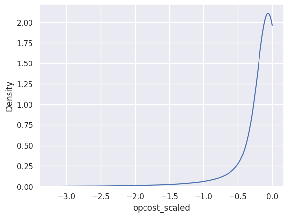
| opcost_scaled | -0.258067 | 1.027769 | 0.00000 | 1.00000 | 0.0 | -0.188721 | -0.059167 | -0.018558 |
panel2.mixture_density("opcost_scaled");
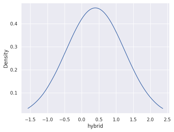
panel2.mixture_density("hybrid");